I’ve always really liked weird album covers from the 70s and 80s (Akiko Yano’s Dolphin is a personal favorite). I like to think that album covers were significantly stranger in the past than they are now (likely untrue). Point being that album covers from specific time periods have a distinct look to them.
For my capstone project, I wanted to see if I could use machine learning techniques to identify these same trends. Can I create a model to learn the decade and the genre of an album cover?
Lessons Learned:
- Training your own neural network is very unwieldy - there are a ton of pre-trained convolutional neural networks out there. This analysis utilizes Graphlab’s but would be curious what the results would be like using TensorFlow’s!
- Balanced samples are key - lessons learned from previous projects can be applied for forever ever. With an over representation of dance songs, and songs from the more recent times, I had to ensure that I was collecting enough from less popular genres, and older time periods.
The Data
Getting the Data - A Frankenstein of Wikipedia and iTunes
In order to get my project going, I needed to pull a large enough data set of album covers from artists 13 musical genres (Comedy, for example, would be left out of as a category) from iTunes. As I took a look at the iTunes API, it seemed pretty easy! It provided all the info I needed for an album, including a link to an album image, genre, and a time period for when the album was released.
Unfortunately, doing any API call in iTunes required an artist to input, which wasn’t helpful for me. The ideal situation would have been to get a randomized list of artists from a specific genre, ranging from the 1980s to present day. iTunes was of no help.
Enter Wikipedia artist lists (example here). For each genre of music, Wikipedia generally has a list of artist names that span from more recent artists to “older” artists. After manually collecting the list of artists per genre that matched up to iTunes genres, I used Wikipedia’s python API, to extract the names from each of these lists.
This artist list of 29,450 was then fed into the iTunes API - now I had 29,450 JSON txt files to deal with. These were read into a dataframe, and cleaned up to include only the relevant data I needed for my analysis.
Key thing to note too is that each artist could have mulitple albums which were nested in the JSON file. The final dataframe contained 137,423 albums, meaning that each artist had an average of 4.7 albums.
Risks/Assumptions
One major issue with this data is the method of collecting the artists from Wikipedia. There’s a lot of reliance on the artist lists being completely representative of nearly 40 years worth of a genre. If this project were to be done again, further exploration could be done on finding another source that would be more comprehensive than Wikipedia (iTunes please have a pull by genre only and not by artist only, kthanks).
There’s also a question of how a genre is determined for a specific artist/album, especially when considering this 40 year long time period. For the sake of simplicity, I assumed that the iTunes genre classification was correct. But, of course, there could be some discrepancy here. Pop is likely particularly tricky, especially over time. Consider an artist like Adele, and her album 19. iTunes has listed this as Pop, R&B / Soul, and Rock. The main genre (which is the one that was utilized in this analysis) would be Pop. At the same time, an artist like DJ Snake, can be categorized as Dance and Pop at the same time. These two artists are also within the same time period!
Another issue that came with this data was the availablity of artists by genre and by decade. Unsurprisingly, there were certain genres that had way more albums vs others. It was more difficult to find Blues albums vs Pop albums. Also, it was much more difficult to find a high volume of albums that were made in the earlier decades vs more recent decades unsurprisingly. 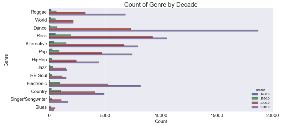
So what does this mean? The train model has to see a balanced sample of genre and decades so that it doesn’t only learn newer dance songs. It also means that we have to select time periods and decades that have enough sample to be able to properly train the model.
The final dataset then had:
- 4 decades: 1980 - 1989, 1990 - 1999, 2000 - 2009, and 2010 - present
- 13 genres: Reggae, World, Dance, Rock, Alternative, Pop, Hip Hop, Jazz, R&B / Soul, Electronic, Country, Blues, Singer/Songwriter
The Target Variable
This part was a bit tricky considering all the above listed risks and assumptions. The ideal situation was to treat the labels of each record as a combination of Decade and Genre in one (e.g. “1980s - Reggae”). But, sample size would just be too small to be able to use this label in a train model. For example, there were only 13 album covers that were categorized as Blues and in the 1980s. This wouldn’t be feasible to create a model that had any sort of predictive power.
The next alternative was to use two different target variables, and create two separate models. Really not ideal (especially given the above risks and assumptions) but it would suffice.
Using the data from the 1980s - present, and across all 13 genres, two models were built with one predicting the genre of an album cover, and another predicting the genre.
This gave me 1,000 album covers per decade (4,000 total), and 800 album covers per genre (10,400 total).
Initial Exploration / Pre-Processing
Proof of Concept
Now that I had all the data and an idea of how to explore my target variables, I wanted to see if this idea could actually work. The key question I wanted to answer in this phase was whether or not there was a qualitiative difference in the way album covers of genres and decades looked.
Thankfully there are many image blending techniques out there that could easily be implemented using Python! I decided to stick with mexitek’s Geek Art github which utilized alpha transparency image blending. You too can replicate his “geek art” via his git.
I decided to use a random sample of 250 album covers per each blended image. Since there were so many album cover samples, if they were all to be blended together, the result would have just been one lovely black useless image.
The results actually showed surprising directional differences between between genres and decades: 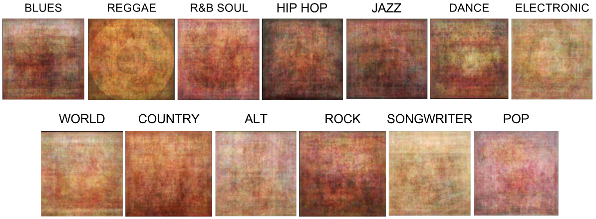
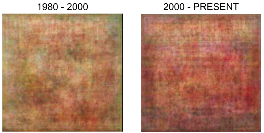
First and foremost, this did directionally prove out that there are differences by genre and decade despite the risk and assumptions listed above. Some other interesting observations:
- Reggae album covers tended to use the vinyl press (or at least in the random sample I used, it was the most distinct element)
- Hip Hop album covers were the darkest out of all the genres
- Pop was the most pink! Kind of weird but fun to know
- Album covers in the earlier decades seemed to be much lighter in color compared to the album covers in more recent decades - maybe color printing techniques are much better now, or people nowadays are more into bold colors?
Thankfully, these blends showed that this concept could work!
Clustering
As a way to possibly combat the overlaps of certain genres, I decided to implement clustering to see if there were any natural clusters that would appear. The KMeans clustering technique ended up yielding the most logical results.
When the clustering was finally complete, the clusters actually didn’t yield any natural defining differences for the genres. Take a look at one of the cluster results for genre: 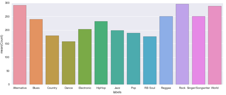
Sad - it’s difficult to see if any particular genres stuck out for one particular label (although directionally Dance and Electronic pretty similar for other clusters - this didn’t yield any better accuracy scores though when they were combined). Unsurprisingly, silhouette score was pretty terrible for this too, at .025.
But, the decade clusters yielded some very directional differences. Silhouette scores weren’t incredibly higher than the poor genre performance (.034), but upon visual inspection, the clusters seemed logical.
The following are the two clusters and the corresponding labels for each decade: 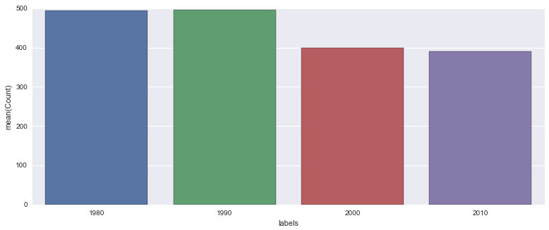
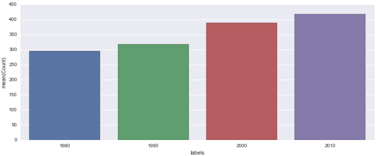
Directionally, it looks like theres a split from pre-2000 and post-2000. Although the silhouette score is relatively low, I moved forward with these clusters because they seemed to make logical sense.
So what now?
This means that the target variables, still remain the 13 genres, and now 2 time periods (vs the original 4) - 1980 to 1999, and 2000 to present.
Model Building
Feature Extraction
Oooooooh images. Features obviously can’t be treated the same as continuous or even discrete data sets. And, there are oh-so-many feature extractors to use for images.
I tried a couple including CV2’s SIFT Features, but, the best performing model used Graphlab’s Deep Feature Extractor. As listed in the Lessons Learned section, this utilizes a pre-trained convolutional neural network to extract features.
Here’s an awesome diagram to show how the pre-trained neural network extracts features for any other image: 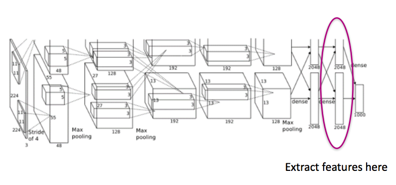 More info can also be found about ImageNet’s deep feature extractor here
There were a few other preprocessing steps that had to be taken into account to actually use this feature extractor.
Here’s the actual code that was used for a genre pull:
#Make sure you've installed graphlab first!
#Installation is relatively painless and can be found here: https://turi.com/download/install-graphlab-create-command-line.html
import graphlab as gl

#All the images are currently in a folder, with the paths as a list in X_test_g.
#The first step is to read each image as a graphlab image
X_test_g_sf = [gl.Image(i) for i in X_test_g]

#Resize each image as a 100 x 100 x 3 image. Although iTunes denotes the album sizes as 100 x 100 x 3, upon examination of individual album covers, some were mis-sized at 97 x 97 x 3 for example. This informs uniformity!
X_test_g_sf = [gl.image_analysis.resize(i, 100, 100, 3, decode=True) for i in X_test_g_sf]

#Fit into a SFrame (Graphlab's version of Pandas dataframe)
X_test_g_sf = gl.SFrame(X_test_g_sf)

#Attach labels to SFrame - also attached the artists just to make ensure that things looked ok
X_test_g_sf["labels"] = y_test_g["updated_genre"]
X_test_g_sf["artists"] = y_test_g["artistName"]

#Activate the deep feature extractor, using the X1 column (this is the column that actually has the image properties)
extractor = gl.feature_engineering.DeepFeatureExtractor(features = 'X1', model='auto')

#Fit to your SFrame and transform!
extractor_g_test = extractor.fit(X_test_g_sf)
features_g_test = extractor_g_train.transform(X_test_g_sf)
Voila, we did it! Here’s what the SFrame looks like now: 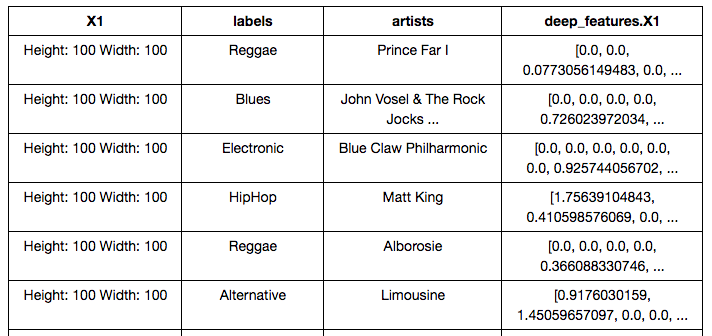
Our deep features are in the “deep_features.X1” column. Now we have two problems though:
- This is in Graphlab’s SFrame format which would be fine and dandy if we would use only Graphlab’s models. But (spoiler alert), we aren’t going to. Scikit Learn has much more flexibility in its models so I had to convert this to a Pandas Dataframe
- The column that we need (the last column on the right) is essentially a list in a single column. We need to extract each of the list items into an individual column
Here’s how we fix those two problems:
#The original SFrame was saved as as a csv. Now its being loaded in as a Pandas Dataframe
df_g_test = pd.read_csv("features_g_test.csv")

#The "list" under the "deep_features.X1" column actually isn't a list - its a string.
#This line converts the list-like string into an actual string
df_g_test["deep_features.X1"] = df_g_test["deep_features.X1"].apply(lambda x: x.replace("[", "").replace("]", "").split())

#When its converted though, it treats each item as a integer rather than a float.
#I wrote a quick little function to convert the list to a float and apply it to the dataframe
def convertint(lizt):
    new_list = [float(i) for i in lizt]
    return new_list
df_g_test["deep_features.X1"] = df_g_test["deep_features.X1"].apply(lambda x: float(i) for i in x)

#Now we can convert each of the items in a list into its own column
new_columns = []

for i in range(len(df_g_test)):
    columns = pd.Series(df_g_test["deep_features.X1"][i])
    new_columns.append(columns)

new_columns = pd.DataFrame(new_columns)
df_g_test_final = pd.concat([df_g_test, new_columns], axis = 1)
Now we have a full image data set with 4,096 features extracted from Graphlab’s Deep Feature Extractor tool. We’re ready to model!
The Model
To first start the model build, I used a train-test split of 80-20, giving me about 8,320 total album covers for genres, and 3,200 album covers for decades to use for a train set.
I ended up testing out the performance of 5 different models inclusive of XGBoost, Gradient Boosted Trees, Neural Networks, KNN and One vs Rest SVM.
I was anticipating both the KNN and SVM to work the best because both classify based off of spatial similarity (loooooooosely). It was unsurprising then that the SVM performed the best out of all the other models.
Through some loose grid-searching, penalty values actually made very little difference in the actual performance of the model. BUT, tuning the kernels actually made a huge impact.
The worst performing kernel was the linear one for both models - when using a polynomial kernel, there was nearly a 10pct pt increase in performance for the genre! For the decade model, it was only increased by 3 pct pt but better than nothing.
So, in summary, the best performing model was a One vs Rest SVM with a polynomial kernel.
On a side note, Gradient Boosted Trees actually ended up outperforming the KNN model and was the second best performing model behind SVM. Those damn trees are always killing it!
The Results
Decades
Because the decade was split up to two labels, the baseline accuracy was .50. The performance of the decade model was .64, 1.3x better than baseline. 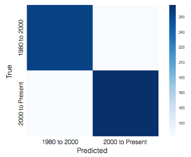
It also looks like the model was not unbalanced - it was nearly equally good at predicting covers that were before 2000 and post 2000.
Genres
Since there were 13 genres which were evenly distributed, it meant that baseline accuracy was .08. The model was performed at .27 accuracy rate. Although not really the highest that it could be, it was about 3.4x higher than the baseline.
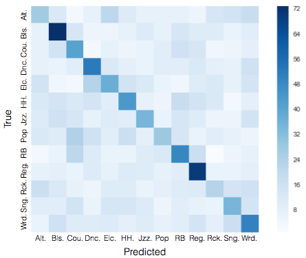
The most well-predicted genres were Reggae, and Blues, at .38 and .39 F-1 Scores, whereas the worst performing was Alternative (.18) and Rock (.17). These results strangely didn’t feel too far off from some of the results we saw in the image blending initial exploration work.
Sample Results
Although the models weren’t the best best best performing, I decided to proceed and see how a few new images would perform.
I first tested out Radiohead’s latest album: 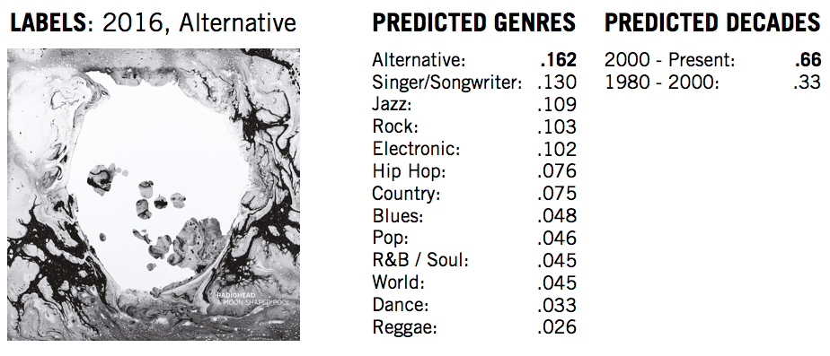
Woah! Surprisingly not bad. The decade model unsurprisingly predicted the proper time period with a high probability. The genre one did predict correctly, albeit not by a far margin. But, even Singer/Songwriter isn’t that far off.
Let’s do some more.
How about Eddie Murphy’s classic, How Could It Be?: 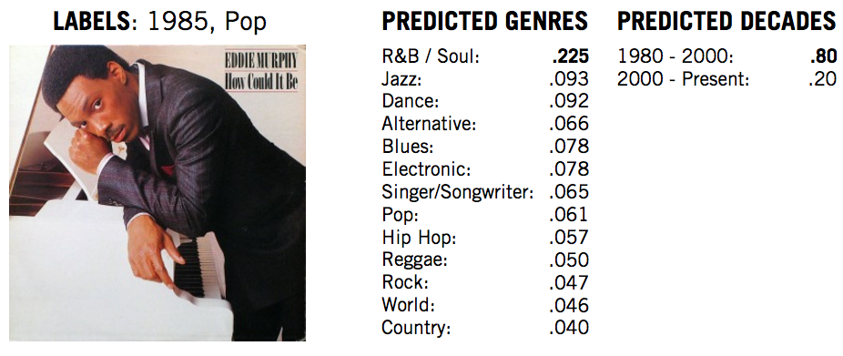
The decade again was overwhelmingly correct, but when looking at the genre, its leaned very heavily towards R&B / Soul. That actually doesn’t feel that far off from an objective stand point, but the proper label of Pop is only predicted at a 6% chance.
Closing Thoughts
Considering that this was the very first time that I had run any sort of machine learning on an image, I was pretty happy that the results were better than baseline. There was definite room for improvement though.
I think the biggest issue here was in the target variable and the data collection. Because the data was split between two models, each model didn’t take into account the other. The Eddie Murphy one I think was a good example and was something that I had hinted at before as well. It was categorized as Pop by iTunes but really that definition could have been very different during 1985. I don’t fully disagree that there were elements of it that could have been categorized as R&B / Soul. And the same could go for the decade model - I’m sure that there were genres that were over represented during specific time periods. Maybe Dance albums, for example, regardless of the time period, would be much more likely to be categorized under 2000s - Present category just because there is an over representation of them during this time.
This could be resolved with an increased sample so that one model could’ve been created which uses a hybrid genre and decade label as previously suggested. Next time!
As this was my first time using a pre-trained convolutional neural network for feature extraction, another way that this model could be built upon would be to test out other models! As I had mentioned earlier, I discovered the Tensorflow pre-trained neural network after the completion of this project. I’d be so curious to see how different the results would be with using a different trained neural network. Any suggestions would also be helpful as well!
As always, if you want to check out the full details of my code, check it out on my git.
I also have a full visual presentation here.
Until next time!