For this week, the goal was to predict the rating of a movie on the IMDb top 250 movie list, and to identify which factors were the most salient in identifying a rating.
Lessons Learned:
- Balanced samples are key - if you want your model to learn each different label, make sure that your training set actually has an evenly distributed amount of labels. You’ll see later how this shakes out unfortunately…
- One metric does not rule them all - this kind of goes along with the above, but just because you have one accuracy number that is pretty good, you need to look at the bigger picture. Not only do you have to compare your accuracy rates against baseline, but its also important to see how accuracy rates differ per label.
The Data Source
Target Variable
The target variable for this exercise was the IMDb rating, which was treated as classification.
Typically, the rating ranges from 0.0 to 10.0, but given that we were focused on the top 250, the minimum in the dataset was 8.0, and the maximum was 9.3. It should be noted that the median of the dataset was 8.3.
As a result, our target variables fell in 3 ranges:
- 8.0 to 8.4
- 8.5 to 9.0
- 8.9 to 10.0
Features
Features were extracted from available information each movies’ IMDb page. The following were chosen based off of their respective assumptions:
- Number of Votes for Rating: assume that these were positively correlated.
- Plot Keywords (pulled all keywords as listed by IMDb): assume that there were specific topics that were of more interest to determine a higher rating.
- Director (could be 1 or 2): assume that specific directors were more likely to create higher ranked movies.
- Top 3 Stars (Actors/Actresses): assume that specific actors/actresses were likely to star in higher ranked movies.
- Year of Release: assume that the age of the movie mattered - classic movies, for example, might have greater credibility, or more recent movies might be fresher, and thus ranked higher.
- Month of Release: assume seasonality mattered (e.g. summer blockbusters or movies closer to awards season).
- Movie Rating: assume that movies that weren’t rated R were more likely to be ranked lower.
- Duration of Movie: assume that length could matter.
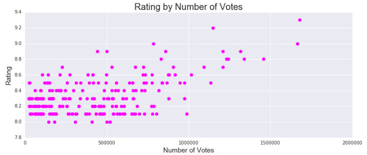
It is worth noting that through initial exploration, Number of Votes appeared to be the most correlated compared to each of the other features:

For text-based features such as Stars, Keywords and Directors, each subset was relatively large. There were 584 individual Stars, 431 Keywords and 167 Directors. So, although there were clear “winners” that were more likely to be in the 250 list (ex: only 5 directors had 7 movies in the list), the length of these features were predicted to have been heavily diluted.
The Final Model
Various tree-based methods were used to develop the model including Decision Trees, Random Forests, Extra Trees, Gradient Boost, Bagged Decision Trees and Extra Trees.
Given apprehensions around the total volume of end features, various feature selection models were tested as well. This included using SelectKBest to identify the top features, and manually extracting features (e.g. plot keywords were left off in one iteration).
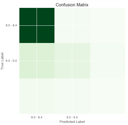
The best performing model based resulted in an accuracy score of .79 , using Gradient Boost model, and all features:

Although the accuracy score was great, it was clear that the sample was waited towards ratings in the lower third of the ratings. Any ratings that were above 8.4 were not predicted by the model in an accurate manner.
Feature Importance
Despite 1,216 total features, the final model was mostly influenced by 1 key features, namely the Number of Votes (as predicted earlier):
| Feature | Relative Importance |
|---|---|
| Number of Votes | .208 |
| Duration | .041 |
| Genre: Sci | .038 |
| Genre: Fi | .037 |
| Keyword: Lake Tahoe | .026 |
| Keyword: Corrupt Politician | .025 |
| Star: Tom Skerritt | .025 |
| Year | .019 |
The fact that Number of Votes was the most salient factor could be a result of mob mentality. Perhaps when a movie is already well-rated, and with a high volume of votes, people are less likely to vote the movie down.
What’s Next?
Although the first iteration of the model had a great accuracy score, with a total of 1,216 features and 250 target variables, it was unsurprising that the result was sub-par.
Most of the next steps should be around reducing the features, and rebalancing the sample to train/test.
Further analysis could be done on refining our feature selection, including reducing plot keywords to a refined few, to reduce the number of features coming from this macro-feature, and potentially increasing the predictability of plot keywords.
Upon refinement, additional features could also be added, including scores from other sites, such as Rotten Tomatoes, or Metacritic.